If I told my younger self that statistics would become cool one day, I'm pretty sure she would have laughed in my face and said, "Statistic, hip? Yeah, right, what BS," and rolled her eyes. I remember how much I hated statistics when I studied pharmacy; I barely passed. I thought statistics was dry and unnecessary. The language in statistics is just odd and a bit counter-intuitive; the bit on inferential statistics is what I'm referring to. For those unfamiliar, there are two categories of statistics: descriptive statistics, which describes data and inferential statistics, which allows you to make predictions ('inferences'). Inferential statistics is counter-intuitive because we start with what we want to prove in hypothesis testing, but what we do is disprove the opposite of what we want to prove; it's rather dumb and confusing, in my opinion. But heck, that's how the statistical cookie crumbles.

I thought my dealing with statistics would end with my pharmacy days, yet fate had a different plan. Years later, during my commerce studies, statistics reared its head again, casting a shadow of dread over me. A melodramatic "Oh noooooo~" might have escaped my lips during class. However, this time, I managed to conquer it with flying colours! My grades were great! BUT, here's the twist: I still didn't understand it. 🙄

You might be scratching your head, wondering, "How in the world did you ace it without getting it?" If you'd asked me then, I would have tried to mask it somehow and not been forthcoming. Today, I'll shamelessly admit that I didn't understand it. As it turns out, research indicates that students who scored As in statistics often performed poorly when tested on the subject the following year. I guess this shows that statistics is not easy to comprehend, and mastery requires multiple attempts, but to be fair, most statistics teachers are too absorbed in mathematics and miss the mark in fostering genuine intuitive understanding.

I now have a better appreciation of statistics and its significance. I've come to recognize that statistics is at the heart of many data-driven innovations such as data analysis, machine learning, finance, business intelligence, healthcare and medicine, artificial intelligence, and much more.

With that said, I will dedicate several blogs to this pivotal topic, focusing on probability distribution. Probability distribution stands as a foundational concept in statistics. Apart from the ubiquitous normal distribution, my grasp of other frequently used distributions remains somewhat poor. I'm aware of their importance, and if I aim to create sophisticated machine learning models (beyond elementary linear regression) and partake in artificial intelligence projects one day, I need to learn and understand these.

So, I'll focus on the basics of probability distribution in this blog. I will dive deeper into some of the more common probability distributions in future blogs.

In this blog, we will look at:

1. What is Probability Distribution and its Link to Statistics?
2. General Properties of Probability Distribution and Notations
3. Discrete vs. Continuous Probability Distributions
4. What are PMF, PDF and CDF?

What is Probability Distribution and its Link to Statistics?

Probability distributions are key ideas that come into play in both probability theory and statistics. Think of probability theory as the tool that helps us understand the chances of various events occurring, while statistics steps in to help us navigate and make sense of data. Now, these probability distributions are the mathematical formulas that show us how likely different outcomes are in an experiment. But guess what? They're not just about predictions; they also have a strong connection with statistics. These probability distributions help us organize data, spot patterns, and find insights. For instance, they arrange messy data, like the heights of people in a group, so we can easily understand and compare different ranges. They can reveal hidden trends in data, making it clear if something happens more often or in a particular way. They can help us discover useful information, like how study habits relate to exam scores, helping us make smarter data-based decisions.

General Properties of Probability Distribution and Notations

General Properties

1. Non-negativity: The chances of something happening can't be negative.
2. Add up to 1: If you add up the chances of all possible things that can happen, the total is always 1.
3. They come in many shapes with different characteristics, and the following key parameters define these:
   a. Mean (µ): The average or central value of a set of data points. It provides a measure of the "central location" of the data.
   b. Variance (σ2): Measures the spread or dispersion of the set of data points. It tells you the average distance squared from the mean.
   c. Standard Deviation (σ): It's the square root of the variance. It gives an idea about the dispersion of the data in the same unit as the data itself.

Notations

Statisticians call numbers that follow a probability distribution "random variables". The notation for random variables that follow a particular probability distribution function is the following:

• "X" represents the random variable
• The tilde, "~" symbol, shows that it follows a probability distribution
• A capital letter signifies the distribution it follows, such as "N" for normal distribution
• Inside the parentheses are the parameters for the distribution, which tells us more about the distribution, like the average (mean µ) and spread (standard deviation σ) of the variables.

For example, if we write X ~ N(µ, σ), it means the random numbers follow a normal distribution with an average of "µ" and a spread of "σ."

As explained, probability distribution shows how likely different numbers are. The notation to describe probabilities is:

p(x) = the likelihood that the random variable takes a specific value of x.

As mentioned above, all the sum of all the probabilities must equal 1, and the change for a particular value is always between 0 and 1.

Example

Let's look at an example involving the heights of students in a school to help you better comprehend the concept of random variables and probability distributions.
Imagine you have a school with many students, and you're interested in studying their heights. You measure the height of each student and record the data.
Our random variable, X, represents the height of a randomly selected student from the school.

Now, let's say that the heights of students in this school roughly follow a normal distribution. The normal distribution is a common pattern where data tends to cluster around a central value and tails off symmetrically on both sides.
Mathematically, we can represent this as follows:
X ~ N(μ, σ)

Here:

• X is the random variable representing the height of a student.
• "~" stands for "follows" or "is distributed as."
• N represents the normal distribution.
• μ is the mean (average) height of all students in the school.
• σ is the standard deviation and gives us an idea of the typical range of heights.

An analogy for the normal distribution could be the shape of a perfectly symmetrical bell. The center of the bell corresponds to the mean height (μ), and as you move away from the center in either direction, the height of the bell decreases, indicating fewer students with extreme heights. The spread of the bell is determined by the standard deviation (σ).

So, when we say the heights of students follow a normal distribution, we mean that most students have heights close to the mean height, and fewer students have heights that deviate significantly from the mean.

Discrete vs Continuous Probability Distribution

Probability distributions can be broadly classified into two main types: discrete probability distributions and continuous probability distributions. These two types capture the different ways probabilities are distributed over the possible outcomes of a random variable.

Discrete Probability Distribution

A discrete probability distribution is a distribution where the random variable can only take on distinct, separate values, typically integers or countable values. Each of these values has an associated probability assigned to it. The probabilities of all possible outcomes must add up to 1.

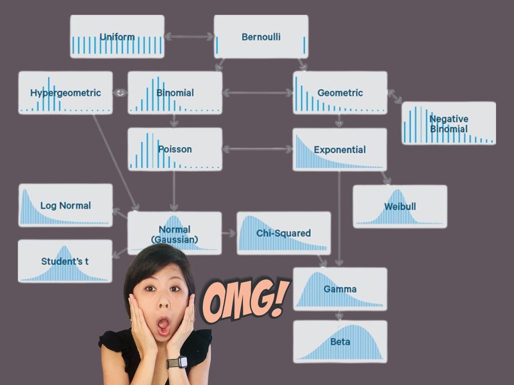
Examples of discrete probability distributions include the binomial distribution, Poisson distribution, and geometric distribution.

For instance, when rolling a fair six-sided die, the outcomes (1, 2, 3, 4, 5, 6) are discrete, and each outcome has a probability of 1/6.

Continous Probability Distribution

A continuous probability distribution is a distribution where the random variable can take on any value within a certain range or interval. Continuous distributions are described using probability density functions (PDFs), and the probabilities are associated with intervals rather than individual values. The total area under the curve of the PDF represents the total probability, which is equal to 1.

Examples of continuous probability distributions include the normal (Gaussian) distribution, exponential distribution, and uniform distribution.

For example, the height of individuals in a population is a continuous random variable. The probability of an individual having a specific height, say exactly 170 cm, is infinitesimally small. Instead, you would look at probabilities over ranges, such as the probability of an individual's height falling between 169 to 171 cm.

In simple terms, think of discrete distributions as dealing with specific things you can count (like dice outcomes), while continuous distributions are about measuring things within a range (like heights or weights).

What is PMF, PDF and CDF

PMF stands for Probability Mass Function.
PDF stands for Probability Density Function.
CDF stands for Cumulative Distribution Function.

These are concepts that apply to various probability distributions. These terms are a bit confusing because they seem similar. It took me a while to remember and understand them. These terms provided a formal mathematical way to describe the distribution of probabilities associated with random variables.

Probability Mass Function (PMF):
• PMF is used for discrete probability distributions (like the binomial or Poisson distribution) where the random variable can only take specific distinct values.
• The PMF gives us the probabilities of each value. It helps us understand the likelihood of getting each particular outcome.

Probability Density Function (PDF):
• PDF is used for continuous probability distributions (like the normal distribution) where the random variable can take on any value within a range.
• It helps us understand the probability of the variable falling within specific intervals.

Cumulative Distribution Function (CDF):
• CDF is used for both continuous and discrete probability distributions.
• The CDF shows how probabilities accumulate as we move along the values of the random variable. It helps us understand the probability of getting a value up to a certain point.

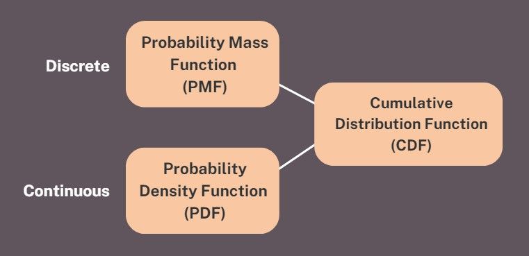
To summarise, probability distributions can be either discrete or continuous. We use the PMF for discrete distributions. For continuous distributions, we use PDF. CDF is relevant to both. The mathematical formulas for PMF, PDF, and CDF vary based on the specific probability distribution. Let me show you. But before I do, be warned that these formulas look intimidating, but don't worry too much about them. I just want to show you that there is a different formula for each distinct probability distribution.

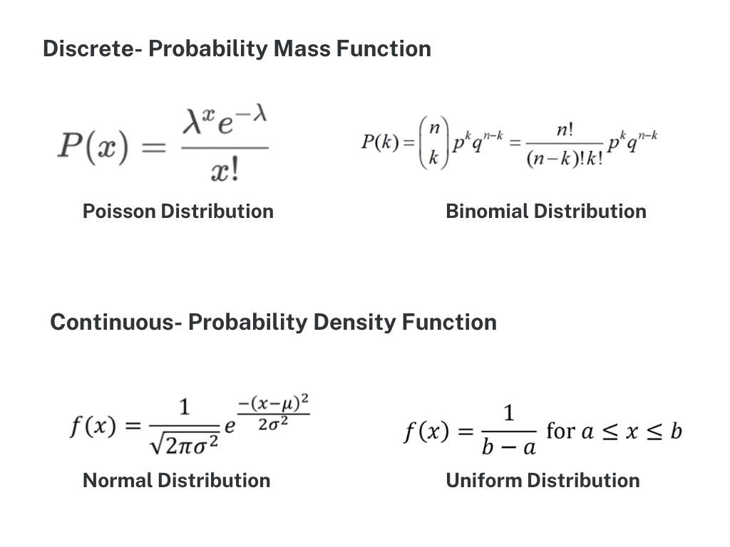
Okay, let's wrap up this lengthy blog. I understand it's a lot to take in. I hope I haven't lost you. These math equations look incredibly daunting, but from my multiple attempts at statistics, I've learned that getting the main idea is more important than remembering every formula. Once you get the concept, the formulas start to make sense. And honestly, I don't stress about memorizing them since I can always look them up when needed. Stay tuned for next week. I'll dive into a specific probability distribution. Any guesses on which one?