Last week, I blogged about probability distributions, providing a beginner's view. I finished the blog by asking for a guess of which distribution I would dive into this week. I bet most would have guessed "normal distribution". Am I right?

Probability tells me that it's an excellent guess. I bet my bottom dollar that if there is one single distribution that people have heard about, it's the normal distribution. Many of us have encountered the concept of normal distribution in some form or another, like discussions about intelligence, talents, or other abilities, hiring processes, or medical research. While I believe many people have heard of it, I also think many people don't know much about it or understand it. Why is it so popular? Why is it called normal? Are all distributions normal? These are some of the questions I had. Admittedly, I didn't think about it the first time I studied statistics because I hated it and could not give two hoots. With a newfound appreciation of stats, I got curious.🤓

So, in this blog, let's look at normal distribution; hopefully, by the end of the blog, you'll appreciate the beauty of it. We will look at:

• What is Normal Distribution?
• Why is Normal Distribution Important?
• Parameters of Normal Distribution
• Properties of Normal Distribution
• Normal Distribution Functions and Z Score

What is Normal Distribution?

This is a normal distribution:

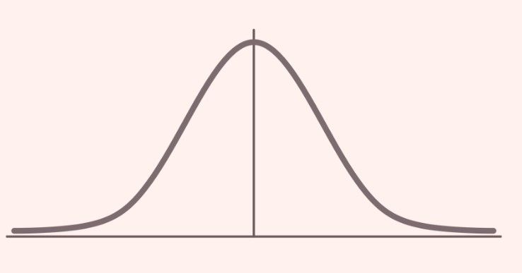
The normal distribution has a few names. It is also known as a bell curve or Gaussian distribution after the German mathematician Carl Friedrich Gauss. Recall in my last week's blog, Probability Distributions for Beginners, there are two overarching types of probability distribution: discrete and continuous, where discrete refers to items that can be counted, and continuous is about measuring things within a range like heights or weights. Normal distribution is a type of continuous probability distribution in which most data points cluster around the middle of the range, while the rest taper off symmetrically toward the extremes.

Why is Normal Distribution Important?

The normal distribution is important for several reasons, especially in fields like statistics and science. Here are a few reasons why it's significant:

Common natural phenomenon: Lots of things in nature follow this normal distribution. For example, the distribution of the wingspans of a large colony of butterflies, the errors made in repeatedly measuring a 1 kg weight, and the amount of sleep you get per night are approximately normal. Many human characteristics, such as height, weight, IQ or examination scores of a large number of people follow the normal distribution. Even random fluctuations in stock prices often show a bell-shaped curve when plotted.

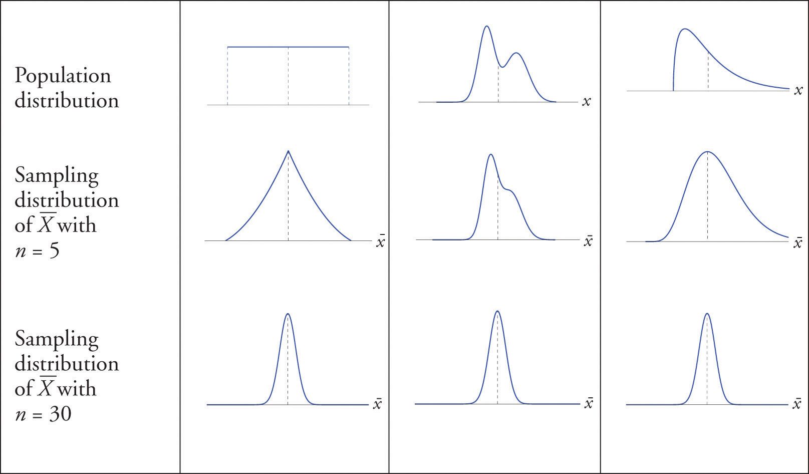
Central Limit Theorem (CLT): I remember being blown off my socks when I first learned this. It's a cool magic rule in statistics, and it's one of the reasons why we see so much of this distribution shape. The CLT states that if you take a sufficiently large number of samples from a population, the samples' means will be normally distributed, even if the population isn't normally distributed.

In simple terms, the CLT tells us that if we take lots of little groups (samples) from a big group (population) and calculate the average for each little group, those averages will form the shape of a bell curve, even if the original big group has a different shape.

Statistical Analysis: The normal distribution has unique mathematical properties, making it a fundamental statistical tool. Many statistical methods and techniques assume that the data follows a normal distribution, simplifying calculations and allowing for more accurate predictions and inferences.
For instance, in many situations, we want to estimate certain parameters of a population, such as its mean (average) and standard deviation (spread). The normal distribution plays a vital role in helping us understand how sample data relates to the larger population and how confident we can be in our estimates.

Parameters of Normal Distribution

In my last blog, I mentioned three parameters common to all distributions, including normal distribution. They are the mean (μ) and the standard deviation (σ). The mean represents the central value or average of the distribution, while the standard deviation measures the spread or variability of the data points around the mean. You might also come across variances (σ2), which is just your standard deviation squared. These parameters define the shape of the normal distribution.

Properties of Normal Distribution

You may be wondering, how are properties different to parameters? Here, we are concerned about the characteristics that make this type of distribution unique and useful:

• Symmetry
• Mean, median, and mode are equal
• Empirical rule
• Skewness
• Kurtosis

Symmetry

The normal distribution is symmetric around its mean. This means the data is equally distributed on both sides of the mean, creating a bell-shaped curve.

Mean, Median, and Mode are Equal

The average (mean), the middle value (median), and the most common value (mode) are all the same in normal distribution. This makes the curve of the distribution look symmetrical.

Empirical Rule

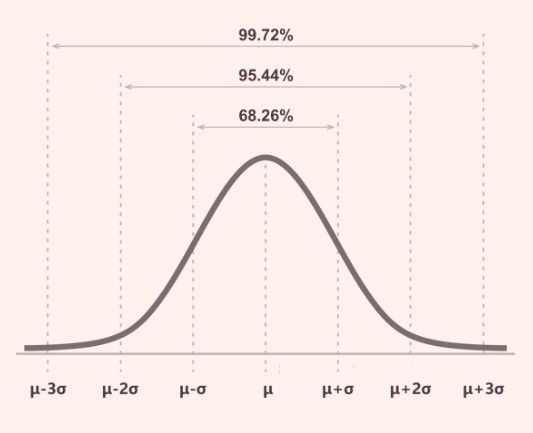
The empirical rule is also known as the 68-95-99.7 rule. Here is what the rule tells us:

• About 68% of the data falls within one standard deviation of the average. The average is the center of the curve, and one standard deviation is the distance from the center towards the edge of the curve. So, if your data is test scores, around 68% of the scores will fall within one standard deviation range.

• About 95% of the data falls within two standard deviations of the average. This means if you go a bit farther from the center (average) – about twice the earlier distance – you'll cover most of the data. So, a big chunk of the scores will be within this larger distance from the average.

• Around 99.7% of the data falls within three standard deviations of the average. Now, if you go even farther out, about three times the earlier distance, you'll include almost all the data. So, only a tiny bit of the data will be outside this wider range.

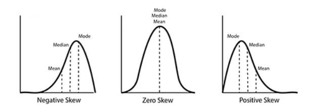
Skewness

Skewness is a measure of the asymmetry of a distribution. It can be left-skewed (negative) or right-skewed (positive). There is no skewness with normal distribution as the data tends to be around a central value with no bias to the left or right.

Kurtosis

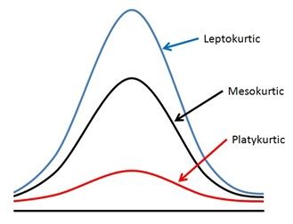
Kurtosis describes the shape of the distribution tails. It quantifies how much data in a distribution deviates from a normal distribution in terms of the heaviness of its tails. High kurtosis indicates heavy tails (more extreme values or outliers), while low kurtosis indicates lighter tails compared to a normal distribution of medium kurtosis.

Here are three terms to describe kurtosis:

• High kurtosis: leptokurtic
• Medium Kurtosis: mesokurtic
• Low Kurtosis: platykurtic

Normal Distribution Functions & Z Score

Ok, we will now venture into the math of normal distribution. Recognizing this is daunting to many, including myself, I'll try to make it as simple as possible.

Normal Distribution Functions

I showed last week there are two functions we need to get ourselves acquainted with.

• Probability density function (PDF)
• Cumulative density function (CDF)

PDF is the math formula that tells you how likely it is to find a particular score. It tells you the likelihood of a certain value occurring.

This formula gives you the relative likelihood of observing a particular value x in the normal distribution. It's important to note that the PDF doesn't give you the actual probability of getting exactly, even though it may appear so, but rather, it gives you the probability of an interval. Remember, the normal distribution is continuous, meaning there are infinitely many possible values within any given range, no matter how small.

CDF is the math formula that helps you keep track of the probabilities as you move along the curve. It tells you the probability that a score is less than or equal to a certain value. So, if you want to know how likely a student's score is below a certain number, the CDF can help you figure that out. Essentially, the formula calculates the area under the curve line up to a particular point.

The relationship between PDF and CDF is that of derivative and integration in calculus, a branch of mathematics that deals with the study of change and accumulation.

To calculate PDF from CDF, we derive—derivate deals with finding the slope of a curve at a specific point. To calculate CDF from PDF, we integrate. Integration is a fancy term that means calculating the area under the curve up to a defined point.

Z Score

The z-score is a handy tool that helps us compare different scores to the average in a standard way. It's like saying, "How many standard deviations is this score away from the average?" A positive z-score means the score is above average, and a negative z-score is below average. A z-score of 0 means the score is exactly at the average.

For example, if you know the average score on a test is 70, and the standard deviation is 10, and a student gets a score of 80, you can calculate the z-score.

The formula is:
z-score = (Score - Mean) / Standard Deviation
So, in this case, the z-score would be (80 - 70) / 10 = 1.
This means the student's score is one standard deviation above the average.

These maths are helpful in statistics because they help us understand and analyze data in a meaningful way.

And that's a wrap! I hope that wasn't too bad and that you better understand and appreciate normal distribution. It is the most common distribution seen and used, but it's not the only type. We will check out a different kind of distribution next week. It won't be obscure but won't be as common as normal distribution. Stay tuned!